Financial stability of national currencies involved in the globalization process requires flexible regulation and control of exchange rate fluctuations dynamics. Government control of currency fluctuations aimed at reducing inflation trends is favorable for economic activity such as forward transactions, business planning, contracts etc. However, in the long term this control prevents national monetary systems from adapting to changeable global environment and can eventually produce large-scale currency crashes. In this paper, the optimal range of exchange rate volatility is evaluated that satisfies both short-scale and large-scale stability requirements of evolution of complex monetary systems. Using two independent methods of volatility estimation, it is shown that deliberate reduction of daily exchange rate fluctuations conducted on a systematic basis inevitably leads to unstable currency dynamics associated with abrupt changes of floating exchange rates and other negative consequences in the long-term. On the other hand, enhanced fluctuations of exchange rate returns described by heave-tailed Pareto-type probability distributions also indicate an unstable behavior of monetary systems.
O.Y. Uritskaya. Evaluation of Optimal Exchange Rate Fluctuations Range by Statistical Temperature Method // Modern Problems and Methods of an Improvement of Government Management.– St.Petersburg: SPbGTU Press, 2004. – p. 378 – 393.

Fig. 1. Method of determining the statistical temperature T and the Pareto index р for currency time series using histograms of logarithmic increments.
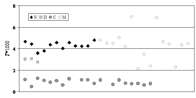
Fig. 2. Values of the statistical temperature T by groups of currencies: N – Economically developed countries: Great Britain, Greece, EU, Canada, New Zealand, Norway, USA, Swiss, Japan, Australia; D – Developing countries with relatively stable monetary systems: Israel, Columbia, Chili, South Africa; C – Unstable Developing countries, prior to crises: Bulgaria, Brazil, India, Kazakhstan, Mexico, Russia, Rumania, Turkey, Ecuador, Indonesia, Malaysia, Singapore, Thailand, Taiwan, Philippines, South Korea; M – the same currencies as in group C after the crisis.

Fig. 3. Examples of normal fluctuations T for time series currency from the group N (top)and nonstationary dynamics of the statistical temperature before and after the currency crises for currency from group C (bottom). The dashed line indicates the lower limit of the fluctuations T for currencies from stable group N.